The Machinery of Generation
TL;DR
This 3-part introduction to flow matching is largely inspired by reference [1].
If you do not have time to complete the full course and companion code, this series is a fast, practical alternative: it distills the core ideas with high-quality visualizations and cleaner code to make the material easier to absorb.
1. Generation as Sampling and Transformation
The starting point of generative modeling is the sampling problem. We are given training samples
$$ z_1,\ldots,z_N \sim p_{\text{data}}, $$where each object is represented as a vector $z \in \mathbb{R}^d$, and the goal is to generate new samples from the same data distribution $p_{\text{data}}$. A useful way to think about this task is the following: generation is not “creating something from nothing,” but sampling through transformation.
More precisely, we first sample from a simple initial distribution
$$ p_{\text{init}} = \mathcal{N}(0, I_d), $$and then transform those easy samples into samples from $p_{\text{data}}$. In this picture, the two key words are:
- Sampling: begin with a point drawn from a simple distribution that we know how to sample from efficiently.
- Transformation: apply a rule that gradually reshapes that simple distribution into the data distribution.
This perspective is the basic machinery of generation. Instead of asking a model to directly output a data sample in one step, we ask it to learn how a cloud of simple random points should move so that, by the end of the process, the cloud matches the geometry of the data distribution. Generation is therefore a transport problem: start from noise, then continuously transform that noise into data.
A Toy Experiment
To make these ideas concrete, consider a two-dimensional toy experiment that we will keep using throughout the article. In this example, the source distribution is
$$ p_{\text{source}} = p_{\text{init}} = p_{\text{simple}} = \mathcal{N}(0, I_2), $$and the target distribution $p_{\text{data}}$ is a symmetric two-dimensional Gaussian mixture with five modes. Because everything lives in $\mathbb{R}^2$, the full generative process can be visualized directly.
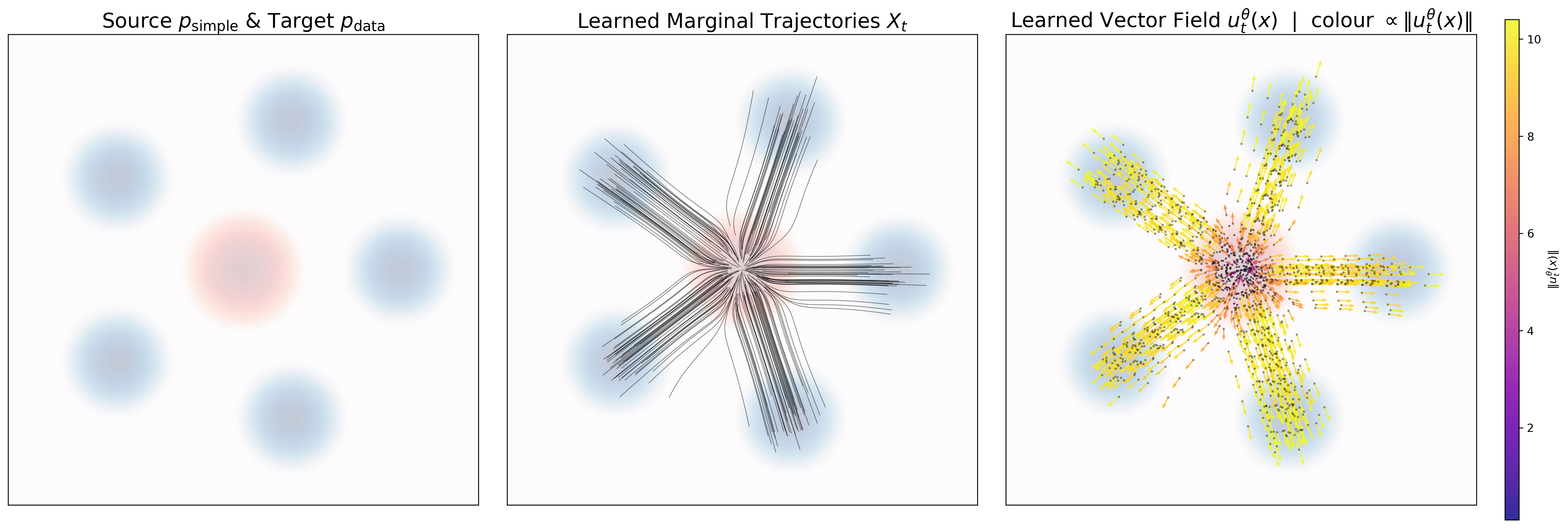
The left panel shows the basic sampling problem. The red density is the source distribution $p_{\text{source}}$, a simple Gaussian that is easy to sample from. The blue density is the target distribution $p_{\text{data}}$, a five-mode mixture representing the data distribution we want to generate from. This panel captures the meaning of sampling and transformation: we start from easy samples, but the goal is to transform them so that they end up distributed like the target data.
The middle panel shows trajectories. Each black curve is the path of one particle that starts from a sampled initial point and evolves over time under the learned ODE. A trajectory therefore records how one sample moves from the source region toward one of the target modes.
The right panel shows the learned vector field $u_t^\theta(x)$. Each arrow gives the instantaneous direction and speed that the model assigns to a point in space, and the arrow color indicates the magnitude $\|u_t^\theta(x)\|$. The vector field is the local motion rule, while the family of all trajectories generated by this rule is the flow. Equivalently, the flow is the global transformation that carries the whole cloud of source samples toward the target distribution.
This toy experiment will serve as the running example for the rest of the discussion. It gives a concrete picture of generation: first sample from $p_{\text{source}}$, then transform those samples by following the learned flow until they match $p_{\text{data}}$.
2. From ODEs to Flow Matching
To make that transformation precise, it is formulated as an ordinary differential equation (ODE). The idea is that the desired transformation is simulated by a time-dependent dynamical system:
$$ \frac{d}{dt}X_t = u_t(X_t), \qquad X_0 = x_0. $$Here $u_t(x)$ is a time-dependent velocity field that tells a particle located at $x$ how it should move at time $t$. This ODE is the mathematical object used to simulate the transformation discussed above. In the language of flow matching, this ODE defines a flow.
Three concepts are fundamental.
First, a trajectory is the solution curve obtained from one initial condition $x_0$. Once we choose the starting point, the ODE traces a path
$$ t \mapsto X_t $$showing how that one particle moves over time.
Second, the vector field $u_t(x)$ is the rule that assigns a velocity vector to every location $x$ at every time $t$. It is the local motion law of the system.
Third, the flow is the family of all trajectories generated by the ODE. If we denote the flow by $\psi_t$, then
$$ \psi : \mathbb{R}^d \times [0,1] \to \mathbb{R}^d, \qquad (x_0,t) \mapsto \psi_t(x_0) \tag{2a} $$For a given initial condition $X_0 = x_0$, a trajectory of the ODE is recovered via
$$ X_t = \psi_t(X_0), $$meaning that the flow maps the initial point $x_0$ to its position at time $t$. Equivalently, the flow satisfies the ODE
$$ \frac{d}{dt}\psi_t(x_0) = u_t(\psi_t(x_0)) \tag{2b} $$with initial condition
$$ \psi_0(x_0) = x_0 \tag{2c} $$This makes the relationship between flow and trajectory very clear: a trajectory is the motion of one initial point, while the flow is the global map that moves every initial point. In other words, each trajectory is one slice of the full flow.
This is exactly the viewpoint needed for generative modeling. We do not want to move only one point; we want to move an entire distribution. If samples from $p_{\text{init}}$ are evolved through the flow, then the final positions of those particles define the generated distribution.
The following is the flow existence and uniqueness theorem from [1]. It states that if
Theorem 3 (Flow existence and uniqueness)
If $ u:\mathbb{R}^d \times [0,1] \to \mathbb{R}^d $ is continuously differentiable with a bounded derivative, then the ODE in (2) has a unique solution given by a flow $\psi_t$. Moreover, $\psi_t$ is a diffeomorphism for every $t$, meaning that the flow is continuously differentiable and has a continuously differentiable inverse $\psi_t^{-1}$.
This is the precise mathematical statement behind the idea that each initial point is transported in one well-defined way. In machine learning, this theorem essentially always applies, because we parameterize $u_t(x)$ with neural networks and treat the required bounded-derivative regularity as part of the modeling setup. Conceptually, this gives the one-to-one correspondence we need between initial points and their transported endpoints. That existence-and-uniqueness result is what makes the transformation a valid generative mechanism rather than an ambiguous motion rule.
However, there is still a practical problem. Even when the vector field $u_t$ is known, the flow $\psi_t$ usually cannot be computed explicitly. For nontrivial vector fields, we do not have a closed-form formula for the solution of the ODE. This is the motivation for introducing a numerical method: to generate samples, we must simulate the ODE rather than solve it analytically.
The simplest such method is the Euler method. If we divide time into small steps of size $h$, Euler’s method replaces the continuous dynamics by the discrete update
$$ X_{t+h} \approx X_t + h\,u_t(X_t). $$The idea is simple: at the current point, read off the velocity from the vector field, take a small step in that direction, and repeat. With many small steps, the discrete trajectory approximates the true continuous trajectory of the ODE. This is why Euler’s method is important for generation: it provides a concrete computational procedure for simulating the transformation from noise to data.
A flow model uses exactly this mechanism. Instead of hand-designing the vector field, we learn a parameterized vector field $u_t^\theta(x)$, typically with a neural network, and define the generative dynamics by
$$ \frac{d}{dt}X_t = u_t^\theta(X_t), \qquad X_0 \sim p_{\text{init}}. $$The model is trained so that the terminal state satisfies
$$ X_1 \sim p_{\text{data}}. $$Once training is complete, sampling from the flow model is straightforward:
- Sample an initial point $X_0 \sim p_{\text{init}}$.
- Choose a time discretization with step size $h$.
- Repeatedly apply the Euler update
- Continue from $t=0$ to $t=1$ and return the final point $X_1$.
So the whole story fits together naturally. Generation can be understood as sampling plus transformation. That transformation can be represented by an ODE, whose induced map is called a flow. Because the flow is usually not available in closed form, we simulate it numerically with Euler’s method. A trained flow model then generates data by starting from simple noise and repeatedly applying Euler steps along the learned vector field until the sample reaches the data distribution.
References
[1] Peter Holderrieth and Ezra Erives. Introduction to Flow Matching and Diffusion Models. 2025. https://diffusion.csail.mit.edu/
[2] Bai-YunHan. Companion code for Introduction to Flow Matching Model. GitHub repository. https://github.com/Bai-YunHan/Companion-code-for-Introduction-to-Flow-Matching-Model